Section 1.4 From problem to model
Loss functions and gradient descent
Consider the linear estimate ŷ = wx + b. The parameters w and b are the slope and intercept. The quantity x could be a normalized volume of requests, and y the corresponding workload in normalized units. The two observations in this section make the arithmetic checkable. A real forecast would need a longer history and a time-aware evaluation.
ŷ = wx + b
L(w, b) = mean[(ŷ − y)²]
One update by hand
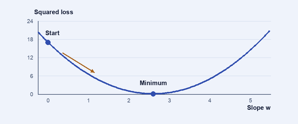
For (x, y) equal to (1, 3) and (2, 5), initialize w and b to zero. The residuals r = ŷ − y are −3 and −5. The mean squared loss is (9 + 25) / 2 = 17. The derivative with respect to w is the mean of 2rx, or −13. The derivative with respect to b is the mean of 2r, or −8. Each negative sign means that a small increase in that parameter reduces the loss at this point, holding the other parameter fixed.
With a step size η of 0.1, the update w ← w − η∂L/∂w gives w = 1.3 and b = 0.8. The new predictions are 2.1 and 3.4, and the loss is 1.685. The explicit calculation shows what the learning rate controls. An oversized step can move beyond the region of improvement even when the gradient is correct.
Choose what the loss penalizes
Squared loss gives increasingly large weight to larger residuals. Absolute error often gives a more direct operational interpretation. A ten-minute error counts ten times as much as a one-minute error in absolute terms. Their squares differ by a factor of one hundred. The training loss and the operational metric can serve distinct purposes. State both before interpreting an improvement.